I’ve just posted an updated version of my paper When Fair Isn’t Fair: Understanding Choice Reversals Involving Social Preferences with Jim Andreoni, Deniz Aydin, Blake Barton, and Doug Bernhiem. This experimental paper shows that our theories of decision making under uncertainty don’t explain behavior when social preferences are involved.

The Context

Let’s say you have $10 to split between two poor households, called A and B. The allocation mechanism we’ll use works as follows:

• You say how to split the money, and then I flip a coin.
• If heads: your split is implemented.
• If tails: your split is ignored, and instead the split ($10, $0) is implemented (that is, all $10 to A).

What allocation do you tell me? Pause and think about it for a second!

Most people say that they would choose the allocation ($0, $10) (all $10 to household B). Note than this means both households will get $5 in expectation. Put another way, your giving all $10 to B if heads is flipped perfectly offsets the chance of all $10 going to A if tails is flipped.

Next, suppose I flip the coin and it comes up heads. Surprise! You can change allocation before implementing if you’d like. What allocation do you tell me now? Again, take a second to think about it.

Most people who said ($0, $10) initially will now switch to ($5, $5). This certainly seems reasonable, as now both households are getting the same payment exactly, not just in expectation.

There’s just one problem: these allocation choices are very difficult to justify with our standard models of decision-making under uncertainty.

Note that your decision before and after the coin flip are actually the same choice from a consequentialist point of view. In the first case, I asked you how you wanted to split the money conditional on heads being flipped. In the second case, I asked you how you wanted to split the money once heads had actually been flipped. So if you are a time-consistent consequentialist, you should say the same thing in both decisions.

Our Design

In this paper, we implemented an experiment that was very similar to the above thought experiment, with just one small tweak: rather than allocating dollars, our subjects allocated 10 lottery tickets to the two households. Another set of 10 tickets was pre-allocated by the computer, and one of the 20 total tickets was eventually chosen as the winning ticket. Whichever household had been assigned that ticket would win $10. In this version, the analogue of finding out the outcome of the coin flip is finding out if the winning ticket is in your set of 10, or the computer’s set of 10. If you’re allocating your 10 tickets without knowing if the winning ticket is among them, we call this the ex ante frame. If you’re allocating your 10 tickets and you do know the winning ticket is among them, we call this the ex post frame.

Importantly, we vary the computer’s allocation of its 10 tickets, so that it is not always (10,0) as in the thought experiment we started off with. For example, the computer might allocate (2,8) in one round, (7,3) in another round, and so on.

Why do the experiment allocating tickets rather than allocating dollars? Because in this case the classical predictions are even starker. Let’s assume you’re an expected utility decision maker. Not only would you need to say the same allocation before and after finding out if the ticket is in your set of 10, but exactly one the the following three statements must be true:

1. You strictly prefer to give all 10 tickets to household A.
2. You strictly prefer to give all 10 tickets to household B.
3. You are indifferent among all ticket allocations.

This hold regardless of the computer’s allocations of tickets. On the other hand, from our thought experiment, we expect to see people choosing to perfectly offset the computer’s allocation ex ante; for example, if the computer’s allocation is (8,2), you might allocated your tickets (2,8). This offsetting behavior we call ex ante equalizing. Conversely, we might see people preferring to divide their tickets evenly. This (5,5) allocation is called ex post equalizing.

Results

So what behavior do we observe? Across decision tasks, we see that people tend to choose the ex ante fair allocation most often in the ex ante frame, and the ex post fair allocation most often in the ex post frame. Figure 1 from the paper makes this very clear:

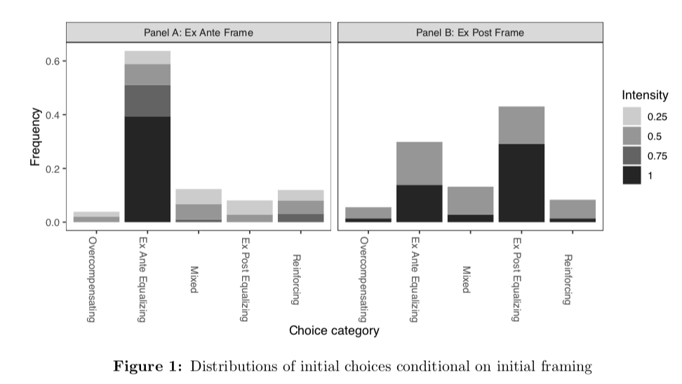
These preferences are strict and do not diminish with experience or exposure. (See the paper for how exactly we know this.)

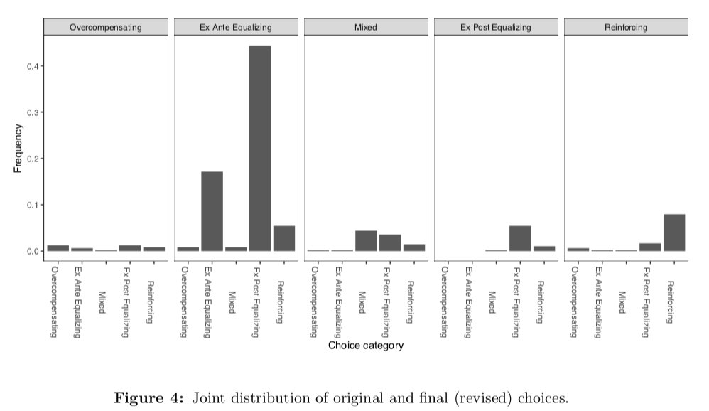
Within decision tasks, we see that choice reversals are common, and they almost always take the form of switching from ex ante equalizing to ex post equalizing. To see this, check out Figure 4 in the paper. In this figure, the panels represent the intial category of the allocation (in the ex ante frame), while the bars within each panel represent the final category (in the ex post frame).

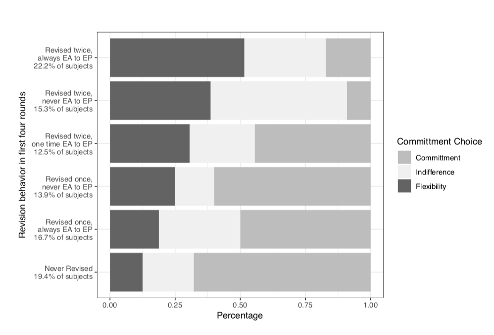
Finally, we ask whether these choice reversals are driven by subjects having consequentialist but time-inconsistent preferences. If this were the case, the subjects who tend to reverse their allocations should demand commitment when offered. Commitment in this case simply means they won’t be asked for their allocation in the ex post frame after having given it in the ex ante frame. However, the subjects who tend to revise often generally choose not to commit themselves:

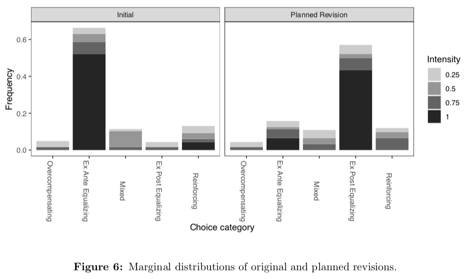
Our second piece of evidence on this question comes from one final treatment. In this treatment, we first asked for allocations in the ex ante frame. Then, before moving to the ex post frame, we asked the subjects if they would like to instruct us to re-allocate their tickets in the case that the winning ticket is in their set of 10. Overwhelmingly, subjects instructed us to re-allocate their tickets in this case to the ex post equalizing allocation, namely (5,5). If reversals were driven by time inconsistency, we instead should have seen subjects sticking with the ex ante fair allocation.

So, what do we think is going on here? Our best guess is that most subjects have non-consequentialist preferences. That is, they may have a procedural definition of fairness which requires choice reversals in this setting. These reversals are not time-inconsistent, since people have preferences over the whole allocation process, not only the outcomes.

If you have any comments, please send me an email, or join the discussion on Twitter

A couple weeks ago, my father-in-law asked for my opinion on the GOP tax bill that had just been rushed through the Senate early in the morning of Saturday, December 2nd. As the reconciled version of the bill seems likely to be passed in both houses today, I thought I’d share the response I sent to my father-in-law.

I should make clear that I am not a macroeconomist, nor am I a public finance expert. Corrections and suggestions are extremely welcome on Twitter! I also wrote this over a week ago, before the reconciliation of the Senate and House versions was completed, so some details may have changed.

My father-in-law sent me this Wall Street Journal opinion piece signed by several high-profile economists, so I started by responding to that article:

The article itself lays out a plausible set of effects of the proposed tax cuts. There is plenty of economic theory to support their claims. However, in economics we like to consider both what the theory says is possible and what the data says has happened in similar situations. In this case, it seems like the authors of the WSJ piece have made some very optimistic assumptions relative to what the data has shown in the past. (For details, see this article by two Harvard economists, Lawrence Summers and Jason Furman.) The last time we made a large cut in the corporate tax rate, business investment actually went down. This time around, it sounds like CEOs plan to spend the tax breaks on dividends for their shareholders, not new innovations. So, there is historical evidence that the tax cuts won’t actually work as intended.

You also asked for my impression of the authors as academics. They are all certainly incredibly smart. I personally was taught by Taylor, who is often mentioned as a potential Nobel Prize winner. However, these guys come from a pretty narrow part of the political spectrum of economists. In fact, most of the Stanford names are associated with the Hoover Institution, which is a conservative think tank on campus. You might get a more representative sample from the University of Chicago’s Economic Experts Panel, which surveys professors from top schools in a variety of subfields of economics. The panel was asked about the tax reform debate: nearly all of them thought the proposed bill would increase the national debt but fail to increase GDP.

It is also worth pointing out that the WSJ authors have made similar predictions in the past. Douglas Holtz-Eakin and Michael Boskin predicted runaway inflation after the last financial crisis; Lawrence Lindsey predicted large deficits during the Obama administration that did not materialize; Glen Hubbard predicted massive job growth after the Bush-era tax cuts. Of course, all of us make predictions that don’t pan out, and it’s a bit unfair for me to cherry-pick the failures. But it does go to show that these folks have been wrong before, and could be wrong again.

I worry that the increase in the deficit would limit the government’s ability to respond to another financial crisis or recession. During busts, the federal budget should run a deficit as the government bails out banks and shores up social support programs. Ideally, it would run a surplus during boom years (which we are probably in right now) to pay back the debt incurred during the downturn. I worry that by adding substantially to the deficit, this tax plan would make it impossible for the government to spend more when it is needed the most. (For more details, see this opinion piece from Forbes.) It also means even more of the budget will have to be allocated to paying back debt.

I also worry that the increase in the deficit could be used as justification for cuts to the social safety next (social security, Medicare, Medicaid, CHIP, etc). In fact, Paul Ryan and others have already suggested that cuts to these programs are necessary to tackle the deficit, which they just made larger by passing the tax cuts. For this reason, it’s really hard not to see the GOP’s agenda as a massive transfer of wealth and resources from poor people to rich people and corporations. As I mentioned above, it’s not clear that these changes are going to spur more growth, but they will make life harder for lots of unlucky Americans.

Finally, the process through which the tax cuts were passed is a bit scary. The bill was rushed through before anyone had a chance to literally even read it, much less do a proper economic analysis. As a result, there were several clear mistakes in the bill, including one which actually raised taxes on a lot of corporations. And now that folks have had a chance to actually analyze the pill, the bi-partisan Joint Commission on Taxation found that it may actually lower GDP. Hopefully these mistakes can be fixed when the bill is reconciled with the Senate version, but the process so far does not exactly inspire confidence.

Inspired by this tweet, I went looking for a graph of state spending on students and on prisoners. I found a couple graphics which I felt could have been done better, so I made my own version.

I found state-by-state data on correctional department spending per prison inmate from vera.org (see figure 4). I found roughly corresponding data on per-pupil K-12 education department spending from the U.S. Census (see table 8).

It is important to note that the prison spending data is from 2010 but the education spending data is from 2013. Comparing across years like this is somewhat dangerous, because the economic and political climates in each state might be very different in those time periods. However, this is the best I could find. Also, there is complete data for only 40 states.

Here is the resulting graph:

Here’s how to interpret the graphs: Each data point is one state. The x-axis is the state’s corrections department spending per prisoner, while the y-axis is the state’s education departments spending per student. If you hover over the state’s data point, you can see the exact numbers for per-prisoner and per-pupil spending, as well as the ratio.

The grey dashed lines indicate where the ratio of per-prisoner to per-student spending would be 1:1, 2:1, 3:1, and 4:1. Note that every state spends more per prisoner than they spend per K-12 student. The highest ratio actually belongs to California, at 5.14:1. The average ratio across the 40 states with complete data is 2.9:1.

The code and data for this graph can be found here.